Reintroduction and the management of our wildlife legacy
Threatened and endangered species can face many hazards including habitat loss, invasive species, disease, and climate change. While habitat conservation, legal protection, and other measures mitigate some of these pressures, local populations may still plummet to a point where local extinctions can occur, ultimately threatening the survival of the species.
Reintroduction is a tool used by wildlife agencies to replenish a local population. Wildlife agencies may restore species by releasing disease-free animals raised in captivity, or by gathering and releasing animals from areas with healthy local populations. Often, the goal of restorative reintroduction is to produce a desired population level without the need for constant intervention. But how many individuals need to be released? Population modeling can help answer this question.
Reintroduction by the numbers
Demographic models with population viability analysis (PVA) capabilities help wildlife managers understand the potential outcomes of different reintroduction strategies. Such models may assess reintroduction strategies using individual-based or population-based analyses. This app uses the latter, in particular a deterministic population matrix model to suggest stage abundances that are immediately aligned with stable population dynamics.
A new tool for determining release abundances
This interactive web-based application has been developed for wildlife managers to identify faunal reintroduction strategies that are immediately aligned with stable population theory. Can flora managers also use this app? Absolutely.
The app aids in reintroduction planning by allowing the user to:
- Enter the elements for a 2-, 3-, 4- or 5-stage population matrix of an iteroparous species of interest,
- Designate the restorative reintroduction goals,
- View the stable proportions of the species of interest,
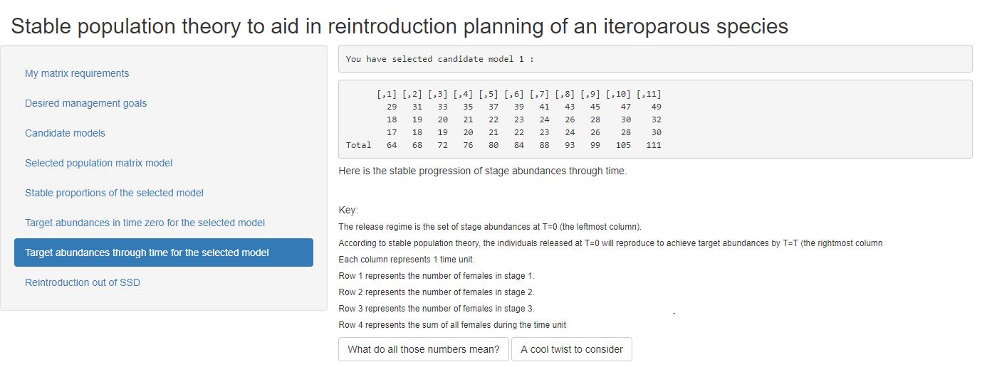
- View the initial release abundances that are mathematically aligned with restoration goals,
- View the theoretical progression of stage abundances through time,
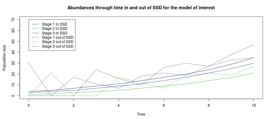
- See what would happen (in a deterministic sense) if individuals are released out of stable-status.
Download the code for use on your own machine
R Studio code for a 2-(St)age StaPOPd population matrix model (Zip archive, 88 KB)
R Studio code for a 3-(St)age StaPOPd population matrix model (Zip archive, 1.4 MB)
R Studio code for a 4-(St)age StaPOPd population matrix model (Zip archive, 247 KB)
R Studio code for a 5-(St)age StaPOPd population matrix model (Zip archive, 5.6 MB)
Would it be handy to have this app for a species with > 5 stages?
Email Dr. Brenda Hanley
The population matrix model
The population matrix model is a stage-structured demographic model that links vital rates in a life history to the population-scale dynamics that they generate (Tuljapurkar, 2008). Also know as the Leslie matrix (age structured; Leslie, 1945) or Lefkovitch (stage structured; Lefkovitch 1965), the population matrix model has been used to enhance understanding and aid management of nearly 8,000 floral and faunal systems across the globe (see Salguero-Gomez et al. 2014, Salguero-Gomez, et al. 2016).
The deterministic population matrix model describes two types of system-level dynamics; ‘asymptotic’ (stable) growth, and ‘transient’ (non-stable) growth. This software suggests reintroduction strategies that are immediately aligned with stable population dynamics with calculations designed to allow populations to theoretically arrive at the predetermined management goals in the desired time frame. Stage abundances that are out of the stable stage distribution (SSD) will produce non-stable, non-patterned transient dynamics (Fox & Gurevitch 2000) that may help or hurt a reintroduction strategy. Transient population oscillations that cause low abundances may alone increase the likelihood of reintroduction failure. Reintroduction of stage abundances in concordance with the SSD ensure that the anthropogenic contribution to the population is aligned with a monotonic population trajectory.
for jennifer's inclusion at the bottom of the more about the model tab.JPG

User Tutorial
Step 1: Enter all the elements of the matrix model for your system of interest. Save your model element entries(by clicking on the save button at the bottom).
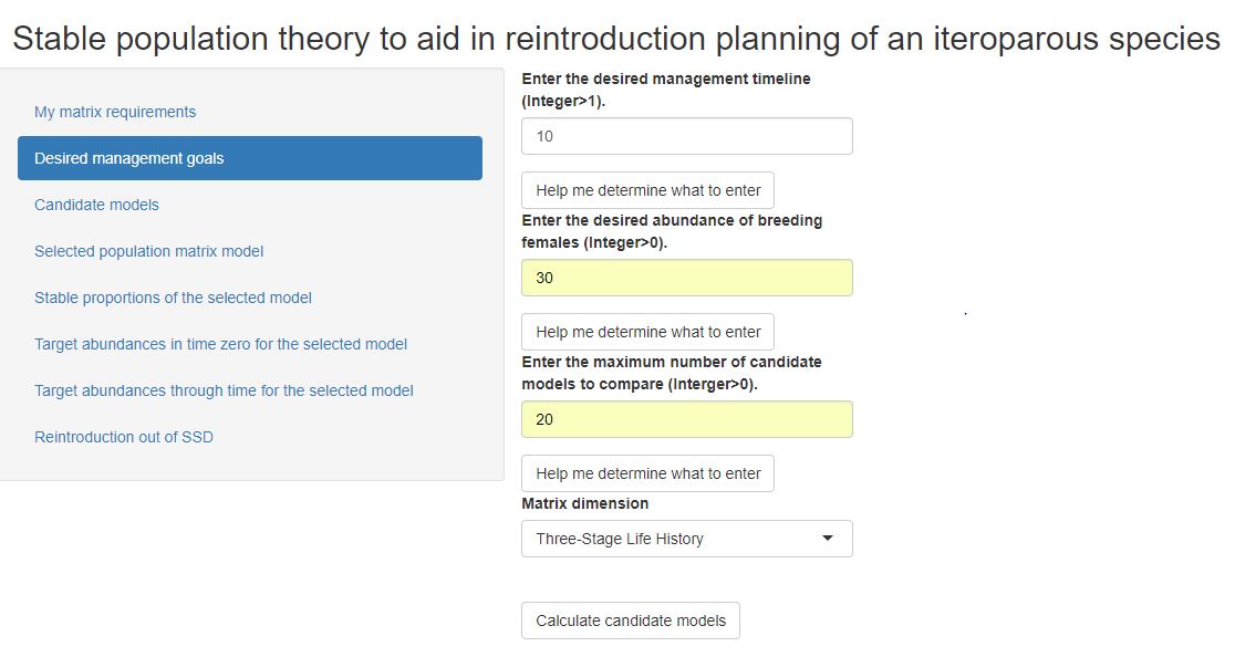
Step 2: Click on the "Desired management goals" tab. Enter your goals, and then click the "Calculate candidate models" button.
Step 3: Click on the "Candidate models" tab. Row 1 will be your model of interest, while the other rows are pre-saved models with similar life history structure and vital rates. Enter the row number corresponding to the model that you wish to investigate. Click on "Calculate detailed information for this model" button. This click will activate all the remaining tabs.
Step 4: View the output on any of the other tabs.
Step 5: Reintroduction out of SSD tab. What if I don't have the proportions of individuals that stable population theory recommends? Enter the abundances that you DO have into the stage-specific boxes. Once all the boxes are filled with an integer value, the deterministic trajectory from those initial conditions will automatically appear on the plot. Maybe the abundances at hand will achieve your goals? Maybe the abundances at hand won't. The app doesn't make any decisions, it just facilitates investigation from the limited perspective of stable population theory.
Want to select a different model to investigate? Return to Step 3.
Want to select a different life history completely, or modify your original model? Return to Step 1.
User Inputs
Model elements: These are the entries of your population matrix model, as parameterized by deterministic, population-scale elements. The elements in the top row are the fertilities, while the elements in the other rows are the transitions. If a fertility or transition does not exist, enter "0". Entries must reflect the formal parameterization of a deterministic, non-density dependent, one-sex stage structured model (e.g. see Caswell, 2001).
Desired unit of time, T: This is an integer above 1, but not more than ~15 (due to technical detail on the math side). The units are consistent with how time in your population matrix model of interest is parameterized. For example, the time unit could be one year, one month, one day, or one hour. This unit is up to you. But the app only takes integers, so please don't type the units!
Desired female abundances at time T: This is an integer greater than 0 that constitutes the target number of breeding females by the end of the management timeline. Type an integer into the box. There is no upper limit.
Stage abundances for viewing trajectories out of SSD: Enter the number of female individuals in each stage that you would like to release. Types integers into each box. These integers must be greater than or equal to 0.
for jennifer.JPG

This app identifies reintroduction considerations through the limited perspective of demographic stable population theory.
In particular, the software omits:
- habitat considerations
- genetic considerations
- disease considerations
- density dependence considerations
- sex ratio considerations
- behavior considerations
- all types of variation (demographic, environmental, sampling)
- weather or climate considerations
- species competition considerations
- migration considerations
- predator considerations
- Release abundances hinge on your timeframe and your desired breeding population. Does the app call for too many to be released? A relaxed timeline or relaxed abundance expectation might be a solution.
- Do problematic discrepancies exist between goal abundances (of all stages) and the carrying capacity of the intended recipient site? Can the site support all the animals in all the stages?
- Do the suggested release abundances constitute a financially realistic captive breeding or live trapping scenario?
- Play around with all the various inputs. Try different combinations of approaches in the context of your species of interest.
- You can scale up or scale down your reintroduction endeavor using stable proportions, and this scaling will indeed maintain stable-status.
for jennifer inclusion.JPG

Please cite this software using:
Hanley, B., Bunting, E., & Schuler, K. 2019. StaPOPd Web Interactive: Interactive software code to "How do we augment the few that remain? Using stable population dynamics to aid reintroduction planning of an iteroparous species" [Software]. Cornell University Library eCommons Repository. https://doi.org/10.7298/d9hg-wa84
Please cite the refereed manuscript using:
Hanley BJ, Bunting EM, Schuler KL. 2019. How can we augment the few that remain? Using stable population dynamics to aid reintroduction planning of an iteroparous species. PeerJ 7:e6873 https://doi.org/10.7717/peerj.6873
The derivations for this app appear in the supplement of the above named work. The mathematical relationship arises from a fundamental result in population demography using population matrix models (Caswell, 2001). All we did was symbolically solve a recursion so these foundational equations could explicitly intake situational management goals, and then make the solution more accessible.
Foundational citations
Caswell, H. (2001). Matrix population models: Construction, analysis, and interpretation. 2nd Ed. Sinauer, Sunderland, Massachusetts, USA. ISBN: 9780878931217
To see just how important population matrix models are to ecology and management, visit:
Salguero-Gómez R, Jones OR, Archer CR, Bein C, de Buhr H, Farack C, Gottschalk F, Hartmann A, Henning A, Hoppe G, Römer G, Ruoff T, Sommer V, Wille J, Voigt J, Zeh S, Vieregg D, Buckley YM, Che-Castaldo J, Hodgson D, Scheuerlein A, Caswell H, Vaupel JW, & Coulson T (2016). COMADRE: a global data base of animal demography, Journal of Animal Ecology, 85(2), 371. DOI: 10.1111/1365-2656.12482
and
Salguero-Gómez R, Jones OR, Archer CR, Buckley YM, Che-Castaldo J, Caswell H, Hodgson D, Scheuerlein A, Conde DA, Brinks E, de Buhr H, Farack C, Gottschalk F, Hartmann A, Henning A, Hoppe G, Romer G, Runge J, Ruoff T, Wille J, Zeh S, Davison R, Vieregg D, Baudisch A, Altwegg R, Colchero F, Dong M, de Kroon H, Lebreton JD, Metcalf CJE, Neel MM, Parker IM, Takada T, Valverde T, Velez-Espino LA, Wardle GM, Franco M, Vaupel JW (2014). The COMPADRE plant matrix database: an open online repository for plant demography. Journal of Ecology, 103(1), pgs 202-218. DOI: 10.1111/1365-2745.12334
and for a helpful individual-based PVA reintroduction model, see:
Vortex: Lacy, R.C., and J.P. Pollak. 2014. Vortex: A stochastic simulation of the extinction process. Version 10.0. Chicago Zoological Society, Brookfield, Illinois, USA.
Other helpful citations
Burgman MA, Ferson S, & Akcakaya HR (1993). Risk assessment in conservation biology. Chapman and Hall. London, United Kingdom.
Crone EE, Ellis MM, Morris WF, Stanley A, Bell T, Bierzychudek P, Ehrlen J, Kaye TS, Knight TM, Lesica P, Oostermeijer G, Quintana-Ascencio PF, Ticktin T, Valverde T, Williams JL, Doak DF, Ganesan R, McEachern K, Thorpe AS, & Menges ES (2012). Ability of matrix models to explain the past and predict the future of plant populations. Conservation Biology, 27(5), 968-978. DOI: 10.1111/cobi.12049
de Kroon, H., Van Groenendael, J., and Ehrlen, J. 2000. Elasticities: a review of methods and model limitations. Ecology. Vol. 81, pgs. 607-618.
Ezard THG, Bullock JM, Dalgleish HJ, Million A, Pelletier F, Ozgul A, & Koons DN (2010). Matrix models for a changeable world: the importance of transient dynamics in population management. Journal of Applied Ecology, 47, 515-523. DOI: 10.1111/j.1365-2664.2010.01801.x
Fox GA & Gurevitch J (2000). Population numbers count: tools for near-term demographic analysis. American Naturalist, 156, 242–256. DOI: 10.1086/303387
Futuyma D (2009). Evolution. 2nd ed. Sinuaer Associates, Inc. Sunderland, Massachusetts, USA.
Gerber BD, & Kendall WL (2016). Considering transient population dynamics in the conservation of slow life-history species: An application to the sandhill crane. Biological Conservation, 200, 228. https://doi.org/10.1016/j.biocon.2016.06.014
Gotelli NJ (2004). A Primer of ecology. Sinuaer Associates, Inc. Sunderland, Massachusetts, USA.
Kissel AM, Palen WJ, Govindarajulu P, & Bishop CA (2014). Quantifying ecological life support: the biological efficacy of alternative supplementation strategies for imperiled amphibian populations. Conservation Letters, 7(5), 441-450. DOI: 10.1111/conl.12093
Koons DN, Grand JB, & Arnold JM (2006). Population momentum across vertebrate life histories. Ecological Modeling, 197, 418-430. DOI:10.1016/j.ecolmodel.2006.03.034
Koons DN, Grand JB, Zinner B, & Rockwell RF (2005). Transient population dynamics: relations to life history and initial population state. Ecological Modeling, 185, 283-297. doi:10.1016/j.ecolmodel.2004.12.011
Koons DN, Holmes RR, & Grand JB (2007). Population inertia and its sensitivity to changes in vital rates and population structure. Ecology, 88, pgs. 2857-2867. https://doi.org/10.1890/06-1801.1
Koons DN, Rockwell RF, & Grand JB (2006). Population momentum: implications for wildlife management. Journal of Wildlife Management. 70, 19-26. https://doi.org/10.2193/0022-541X(2006)70[19:PMIFWM]2.0.CO;2
Lacy RC (2000). Structure of the VORTEX simulation model for population viability analysis. Ecological Bulletins, 48, 191-2003. DOI: 10.2307/20113257
Lefkovitch LP (1965). The study of population growth in organism groups by stages. Biometrics, 21, 1-18. DOI:10.2307/2528348
Leslie PH (1945). On the use of matrices in certain population mathematics. Biometrika, 33, 183-212. https://doi.org/10.1093/biomet/33.3.183
McDonald JL, Stott I, Townley S, & Hodgson DJ (2016). Transients drive the demographics of plant populations in variable environments. Journal of Ecology, 104, 306-314. DOI: 10.1111/1365-2745.12528
Morris WF & Doak DF (2002). Demographic PVAs: Using projection matrices to assess population growth and viability. – In: Quantitative conservation biology: theory and practice of population viability analysis. Sinauer Associates Inc., 215-250.
Pacioni C & Mayer F (2017). VORTEXR: an R package for post Vortex simulation analysis. Methods in Ecology and Evolution, 8, 11. DOI: 10.1111/2041-210X.12786
R Core Team. (2018). R: A language and environment for statistical computing. R Foundation for Statistical Computing, Vienna, Austria. URL https://www.R-project.org/ [accessed 12 Oct 2018]
R Shiny. (2018). Shiny. Web Application Framework for R. URL http://shiny.rstudio.com [accessed 12 Oct 2018]
RStudio Team. (2015). RStudio: Integrated Development for R. RStudio, Inc., Boston, MA URL http://www.rstudio.com/ [accessed 12 Oct 2018]
Starfield AM & Bleloch AL (1986). Building models for conservation and wildlife management – MacMillan. South Dakota State University, Brookings, SD, USA.
Starfield AM (1997). A pragmatic approach to modeling for wildlife management. Journal of Wildlife Management. 61, 261-270. DOI: DOI: 10.2307/3802581
Stott I, Hodgson DJ, & Townley S (2010). Beyond sensitivity: nonlinear perturbation analysis of transient dynamics. Methods in Ecology and Evolution. 3, 673-684. DOI: 10.1111/j.2041-210X.2012.00199.x
Stott I, Hodgson DJ, & Townley S (2012). Popdemo: an R package for population demography using projection matrix analysis. Methods in Ecology and Evolution, 3, 797-802. DOI: 10.1111/j.2041-210X.2012.00222.x
Stott I (2016). Perturbation analysis of transient population dynamics using matrix projection models. Methods in Ecology and Evolution, 7, 666-678. DOI: 10.1111/2041-210X.12543
Tuljapurkar S (1997). Demographic uncertainty and the stable equivalent population. Mathematical Computational Modeling, 26(6), 39-56. https://doi.org/10.1016/S0895-7177(97)00168-4
Tuljapurkar, S. (2008). Stable population theory. In - The New Palgrave Dictionary of Economics. 2nd Edition. (eds). Steven N. Durlauf and Lawrence E. Blume. Palgrave Macmillan, United Kingdom.
Wiedenmann J, Fujiwara M, & Mangel M (2009). Transient population dynamics and viable stage or age distributions for effective conservation and recovery. Biological Conservation, 142, 2990-2996. DOI:10.1016/j.biocon.2009.07.031


